29

A feature of latex is that you can "program your document". You can do this by using TeX/LaTeX directly (remember that it is Turing complete) or by other languages like lua or python (especially sage) or other languages where a package exists to use that code to program in latex. In particular TeX or lua is heavily used when developing a new package.

However I want examples which show this "paradigm" from the point of view of a user.

The examples should be at best real use cases. For example if you have made use of this paradigm to set up a nice document using loops and other programming features in the past and you are (a bit) proud of it, please post it. It is also welcome if you come up with new examples just for this question.

Please post the source code and the result. It would be nice if you could pay attention to commented, clean (perhaps elegant) source code.

I think great answers to this would be both educational and inspiring and would also provide further arguments why to prefer LaTeX over other software for example some text-processors...

12
  • 2
    Point of view of a user is precisely avoiding such kind of programming no? That's why we have La over TeX.
    – percusse
    Commented Dec 28, 2014 at 21:00
  • 3
    @percusse An example from the point of a user would be for instance this one: tex.stackexchange.com/questions/53458/… I think packaging and programming for the user are not exclusive.
    – student
    Commented Dec 28, 2014 at 21:04
  • 1
    I export marks and feedback from calc, run a couple of bash scripts to produce 2 .dat files, and then use textmerg to loop through the .dat files to create feedback sheets and address labels. Saves keep writing stuff out when completing end-of-module paperwork.
    – cfr
    Commented Dec 28, 2014 at 21:11
  • 2
    See stackoverflow.com/q/2968411/315213 for an older version of this question on StackOverflow. Commented Dec 29, 2014 at 8:28
  • 1
    @LoopSpace Yes, this would count if you use some programming to make things with those packages, see the example by cryingshadow. However just because inside the packages programming techniques are used (like in most packages), it does not.
    – student
    Commented Dec 29, 2014 at 15:46

8 Answers 8

22

I'm not sure if this is appropriate, but in the distant past, before I was aware of packages like Tikz, I wrote some routines for performing arithmetic operations in plain TeX using dimensions (plain TeX can do this also, but discards remainders).

I apologize for the, most likely, horrendous code.

Here are some utility macros (these are used for other routines I've made. Some of these may not be used in what follows):

    \catcode`\!=11               % To help prevent macros being redefined in the main document
    \catcode`\@=11               %

    \def\dlap#1{\vbox to 0pt{#1\vss}}      \def\ulap#1{\vbox to 0pt{\vss#1}}
    \def\chlap#1{\hbox to 0pt{\hss#1\hss}} \def\cvlap#1{\vbox to 0pt{\vss#1\vss}}
    \def\clap#1{\chlap{\cvlap{\hbox{#1}}}}

    %  List/token manipulatuion routines
    %  See The TeXboox, pg. 378-379
    %
    \toksdef\ta=0 \toksdef\tb=2 %
    \long\def\leftappend#1\to#2{\ta={\\{#1}}\tb=\expandafter{#2}%
             \edef#2{\the\ta\the\tb}}
    \long\def\rightappend#1\to#2{\ta={\\{#1}}\tb=\expandafter{#2}%
             \edef#2{\the\tb\the\ta}}
    \def\concat#1=#2&#3{\ta=\expandafter{#2}\tb=\expandafter{#3}%
             \edef#1{\the\ta\the\tb}}
    \def\lopl#1{\expandafter\lopoffl#1\lopoffl#1\to}      
    \long\def\lopoffl\\#1#2\lopoffl#3\to{\gdef#3{#2}{#1}}
    \def\lop#1\to#2{\expandafter\lopoff#1\lopoff#1#2}     
    \long\def\lopoff\\#1#2\lopoff#3#4{\def#4{#1}\def#3{#2}}
    \def\alop#1\to#2{\expandafter\alopoff#1\alopoff#1#2}     
    \long\def\alopoff\\#1#2\alopoff#3#4{\global#4=#1\def#3{#2}}
    \def\select#1\of#2\to#3{\def#3{\outofrange}%
        \long\def\\##1{\advance#1-1 \ifnum#1=0 \def#3{##1}\fi}#2}
    \def\assign#1\of#2\to#3{%
        \long\def\\##1{\advance#1-1 \ifnum#1=0 \global#3=##1\fi}#2}
    \def\card#1\to#2{#2=0 \long\def\\##1{\advance#2 by1 }#1}
    \def\outofrange{}
    \def\sevenea{\expandafter\expandafter\expandafter\expandafter
        \expandafter\expandafter\expandafter}              
    \def\length#1\to#2{{\count0=0 \getlength#1\end \global#2=\the\count0 }}
    \def\getlength#1{\ifx#1\end \let\next=\relax
        \else\advance\count0 by1 \let\next=\getlength\fi \next}
    {\catcode`p=12 \catcode`t=12 \gdef\GrabI#1.#2pt{#1} \gdef\GrabD#1.#2pt{#2}}
    \def\ItPart#1{\expandafter\GrabI\the#1}
    \def\DecPart#1{\expandafter\GrabD\the#1}
\def\GRLABEL#1(#2,#3){\ulap{\vbox{\rlap{\kern#2\relax#1}\kern#3\relax}}}

Here are the (very much unoptimized) math routines:

    %%%%%%%%%%%%%%%%%%%%%%%%%%%%%%%%%%%%%%%%%%%%%%%%%%%%%%%%%%%%%%%%%%%%%%%%%%%%%%
    %%%%%%%%%%%%%%%%%%%%%%%%%%%%%%%%%%%%%%%%%%%%%%%%%%%%%%%%%%%%%%%%%%%%%%%%%%%%%%
    %                                                                            %
    %                            MATH ROUTINES                                   %
    %                                                                            %
    %%%%%%%%%%%%%%%%%%%%%%%%%%%%%%%%%%%%%%%%%%%%%%%%%%%%%%%%%%%%%%%%%%%%%%%%%%%%%%
    %%%%%%%%%%%%%%%%%%%%%%%%%%%%%%%%%%%%%%%%%%%%%%%%%%%%%%%%%%%%%%%%%%%%%%%%%%%%%%

    \newcount\!!!     
    \newdimen\t@mpthree
    \newdimen\t@mp
    \newdimen\t@mptwo
    \newcount\k@
    \newcount\j@
    \newcount\l!
    \newcount\R@M
    \newcount\S!GN
    \newtoks\@ns
    %
    %
    %   Multiplication/Division routines
    %
    %
    \def\MulDim#1#2\to#3{#3=\ItPart{#1}.\DecPart{#1}#2}
    \def\DivDim#1#2\to#3{{\l!=\ItPart{#1}\DecPart{#1}\j@=\ItPart{#2}\DecPart{#2}% 
        \ifdim#1=0.0pt\global#3=0.0pt    %added global 0ct 16 2010
        \else
             \ifnum\l!<0 \ifnum\j@<0 \S!GN=1 \l!=-\l! \j@=-\j@ \else\l!=-\l! \S!GN=-1 \fi
                   \else\ifnum\j@<0 \j@=-\j@ \S!GN=-1 \else\S!GN=1 \fi
        \fi
        \sevenea\length\DecPart{#2}\to\k@ \sevenea\length\DecPart{#1}\to\!!! 
        \ifnum\!!!<\k@ \advance\k@ by-\!!! 
              \multiply\l! by\ifcase\k@ 1 \or10 \or100 \or1000 \or10000 \or100000\fi
        \else\advance\!!! by-\k@     
             \multiply\j@ by\ifcase\!!! 1 \or10 \or100 \or1000 \or10000 \or100000\fi  
        \fi
        \k@=\l! \divide\k@ by \j@ \@ns=\expandafter{\the\k@.}%
        \R@M=\k@ \multiply\R@M by-\j@ \advance\R@M by \l!
        \G@TN@XT\G@TN@XT\G@TN@XT\G@TN@XT\G@TN@XT\G@TN@XT\G@TN@XT  
            \global#3=\the\@ns pt \global\multiply#3 by \S!GN \fi}}
    \def\G@TN@XT{%
        \ifnum\R@M=0
        \else\multiply\R@M by 10 \k@=\R@M \divide\k@ by \j@  
             \edef\tmp{\the\@ns \the\k@}\@ns=\expandafter{\tmp}%  
             \multiply\k@ by\j@ \advance\R@M by -\k@
        \fi}
    \def\MidPoint#1#2\to#3{\t@mp=#2\advance\t@mp-#1\divide\t@mp by2%
                                                          \advance\t@mp#1#3=\t@mp}
    %
    %  Cosine\Sin routine
    %
    %
    \def\Cos#1\to#2{\S!GN=1\ifdim#1<0.0pt#2=-#1\else#2=#1\fi
        \loop\ifdim#2>6.2831853072pt\advance#2-6.2831853072pt\repeat
        \ifdim#2<4.7123889804pt\ifdim#2>1.5707963268pt\advance#2-3.14159265pt%
                                                                  \S!GN=-1 \fi\fi
            \ifdim#2<6.2831853072pt\ifdim#2>4.7123889804pt\advance#2-6.2831853072pt%
                                                                  \fi\fi                                                                                                
        \MulDim#2#2\to\t@mp
        #2=.0178571\t@mp\advance#2-1pt
        \MulDim\t@mp{#2}\to{#2}#2=0.033333333 #2\advance#21pt
        \MulDim\t@mp{#2}\to{#2}#2=0.083333333 #2\advance#2-1pt
        \MulDim\t@mp{#2}\to{#2}#2=0.50000 #2\advance#21pt\global #2=\S!GN #2}
    \def\Sin#1\to#2{\t@mptwo=#1\advance\t@mptwo by-1.5707963268pt\Cos\t@mptwo\to{#2}}
\catcode`\!=12
\catcode`\@=12 

(Incidentally, I was particularly proud of using a "seven \expandafter" in the \DivDim routine. I wonder if it's needed...)

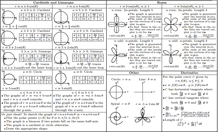
One application of these routines is to produce graphs. Here are some macros I made to produce polar curves:

\newcount\iii
\newdimen\tempx
\newdimen\tempy
\newdimen\Slope
\newdimen\temp
\newdimen\temptwo
\newdimen\tempthree
\newdimen\tempfour
\newdimen\cinc
\newdimen\x
\setbox46\hbox{{\kern-.1pt\vrule width.6 pt height .4pt depth0pt}}
\setbox48\hbox{{\kern-.1pt\vrule width.6 pt height .4pt depth0pt}}
    %
    %    Sketch the graph of r=#1(#2+#3 cos(#4 \theta) from theta = #5 to #6.  #7 controls the resolution (higher for finer resolution) )
    %    The produced size will be r_max=#1*(#2+#3) points.  Arguments are numbers (no ''pt'')
    %
    \newdimen\ct\newdimen\st
    \def\CosPolarGraph#1#2#3#4#5#6#7{% 
          \x=#5 pt  
                \temptwo=#7pt \ifdim\temptwo<0 pt \temptwo=-\temptwo\fi \cinc=.01pt \DivDim\cinc\temptwo\to\cinc 
                \temp=#4pt 
                \tempthree=#3 pt
          \loop\ifdim\x<#6pt%
                     {\Cos{\x}\to\ct 
                        \Sin{\x}\to\st  
                        \MulDim\temp\x\to\tempfour              %
                        \Cos\tempfour\to\tempfour               %   compute r
                        \MulDim\tempfour\tempthree\to\tempfour  %
                        \tempthree=#1 pt                        % 
                        \advance\tempfour by #2 pt              % 
                        \MulDim\tempfour\tempthree\to\tempfour  %
                        \MulDim\st\tempfour\to\tempy
                        \MulDim\ct\tempfour\to\tempx
                        \GRLABEL{\copy46}(\tempx,\tempy)}%
                      \advance\x by \cinc
           \repeat} 
    %%%%%%%%%%%%%%%%%%%%%%%%%%%%%%%%%%%%%%%%%%%%%%%%%%%%%%%%%%%%%%%%%%%%%%%%%%%%%%%%%%%%%%%%%%%%%%%%%%%%%%%%%%%%%%%%%%%%%%%%%%%%%%%%%%%%%%%%
    %
    %
    %    Sketch the graph of r=#1(#2+#3 sin(#4 \theta) from #5 to #6.  #7 controls the resolution (higher for finer resolution) )
    %    The produced size will be r_max=#1*(#2+#3) points.  Arguments are numbers (no ''pt'')
    %                                                                       
    \def\SinPolarGraph#1#2#3#4#5#6#7{%  
          \x=#5 pt  
                \temp=#7pt \ifdim\temp<0 pt \temp=-\temp\fi \cinc=.01pt \DivDim\cinc\temp\to\cinc 
                \loop\ifdim\x<#6pt%
                     {\temp=#4pt
                      \MulDim\temp\x\to\tempfour              %
                        \Sin\tempfour\to\tempfour               % 
                        \temp=#3 pt                             %   compute r
                        \MulDim\tempfour\temp\to\tempfour       %
                        \temp=#1 pt                             % 
                        \advance\tempfour by #2 pt              % 
                        \MulDim\tempfour\temp\to\tempfour       %%%%%
                        \Sin{\x}\to\temp
                        \MulDim\temp\tempfour\to\tempy           
                        \Cos{\x}\to\temp                            
                        \MulDim\temp\tempfour\to\tempx           
                        \GRLABEL{\copy46}(\tempx,\tempy)}%
                      \advance\x by \cinc
           \repeat}     
    %%%%%%%%%%%%%%%%%%%%%%%%%%%%%%%%%%%%%%%%%%%%%%%%%%%%%%%%%%%%%%%%%%%%%%%%%%%%%%%%%%%%%%%%%%%%%%%%%%%%%%%%%%%%%%%%%%%%%%%%%%%%%%%%%%%%%%
    %
    % Archimedian Spiral. Sketch the graph of r=#1 * \theta from #2 to #3  
    %
    %                           
    \def\Spiral#1#2#3{% 
          \x=#2 pt% 
                \cinc=.01pt%  
                \loop\ifdim\x<#3pt%
                     \temp=#1pt
                      \MulDim\temp\x\to\tempfour                   % Compute r
                        {\Sin{\x}\to\temp
                        \MulDim\temp\tempfour\to\tempy                
                        \Cos{\x}\to\temp                            
                        \MulDim\temp\tempfour\to\tempx                
                        \GRLABEL{\copy46}(\tempx,\tempy)}%
                      \advance\x by \cinc
           \repeat}                                                                                 
    %%%%%%%%%%%%        

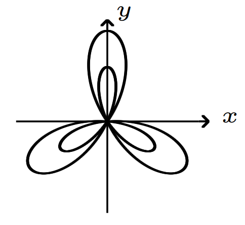
Here is some sample output (which looks much better than the screen capture would indicate)

enter image description here

The command \SinPolarGraph{8}{.5}{-2}{3}{0}{6.28}{2}, for example, produced the "nested rose" in the "Other" box (TeX needs to be in horizontal mode when \SinPolarGraph is called). Here is a close up:

enter image description here

All done using only plain TeX!

19

Plain TeX, a suitable document for the season. The document consists of two nested recursive loops to generate the text.

\let~\catcode~`76~`A13~`F1~`j00~`P2jdefA71F~`7113jdefPALLF
PA''FwPA;;FPAZZFLaLPA//71F71iPAHHFLPAzzFenPASSFthP;A$$FevP
A@@FfPARR717273F737271P;ADDFRgniPAWW71FPATTFvePA**FstRsamP
AGGFRruoPAqq71.72.F717271PAYY7172F727171PA??Fi*LmPA&&71jfi
Fjfi71PAVVFjbigskipRPWGAUU71727374 75,76Fjpar71727375Djifx
:76jelse&U76jfiPLAKK7172F71l7271PAXX71FVLnOSeL71SLRyadR@oL
RrhC?yLRurtKFeLPFovPgaTLtReRomL;PABB71 72,73:Fjif.73.jelse
B73:jfiXF71PU71 72,73:PWs;AMM71F71diPAJJFRdriPAQQFRsreLPAI
I71Fo71dPA!!FRgiePBt'el@ lTLqdrYmu.Q.,Ke;vz vzLqpip.Q.,tz;
;Lql.IrsZ.eap,qn.i. i.eLlMaesLdRcna,;!;h htLqm.MRasZ.ilk,%
s$;z zLqs'.ansZ.Ymi,/sx ;LYegseZRyal,@i;@ TLRlogdLrDsW,@;G
LcYlaDLbJsW,SWXJW ree @rzchLhzsW,;WERcesInW qt.'oL.Rtrul;e
doTsW,Wk;Rri@stW aHAHHFndZPpqar.tridgeLinZpe.LtYer.W,:jbye
5
15

Here is the invitation to my 30th birthday that I did using two foreach loops in TikZ. The text is in German (and the main message is "30 years of madness"). Enjoy! ;)

\documentclass{article}

% use German input
\usepackage[utf8]{inputenc}
\usepackage[T1]{fontenc}
\usepackage{ngerman}

% play with colors
\usepackage{xcolor}

% this should be a 10x15cm postcard
\usepackage[paperwidth=15cm,paperheight=10cm,margin=0pt]{geometry}

% for using a math symbol
\usepackage{amssymb}

% for importing photos
\usepackage{graphicx}

% for drawing the main picture (the spiral) 
\usepackage{tikz}
\usetikzlibrary{positioning}

% the page should be filled with a background color
\pagestyle{empty}
\pagecolor{blue!40}

% the spiral evolves by the number of years
\newcounter{myyear}
% smaller than 7 is not readable
\setcounter{myyear}{7}

% output the current year and advance the counter
\newcommand{\myyear}{\arabic{myyear}\stepcounter{myyear}}

\begin{document}

\vspace*{-2mm}

\begin{center}
{\Huge \textit{\textbf{\textcolor{white}{Einladung}}}}

\vspace*{-8mm}

\hspace*{-15mm}
\begin{tikzpicture}
% draw a shaded spiral using polar coordinates
\foreach[count=\y from 1] \x in {0, 1, ..., 29}{
  \shadedraw[left color=yellow,right color=red, draw=black] (\x r:0.004*\x*\x) -- (\y r:0.004*\y*\y) -- (\y r:0.005*\y*\y) -- (\x r:0.005*\x*\x) -- cycle;
}
% add the years half way
\foreach[count=\y from 1] \x in {6.5, 7.5, ..., 28.5}{
  \node at (\x r:0.0045*\x*\x) {\fontsize{\y pt}{\y pt}\selectfont\textcolor{white}{\myyear}};
}
% now add some pictures and text around the spiral
\node (a28) [xshift=-5.7cm,yshift=1.9cm,rotate=-10] {\includegraphics[height=4cm]{tom28.jpg}}
  edge[draw=black, shorten >=5pt, thick] (27.5 r: 0.0045*27.5*27.5);
\node (a8) [right=8 of a28, rotate=10] {\includegraphics{tom8.jpg}}
  edge[draw=black, thick] (7.5 r: 0.0045*7.5*7.5);
\node (a18) [below=0.1 of a8, rotate=-10] {\includegraphics{tom18.jpg}}
  edge[draw=black, shorten >=5pt, thick] (17.5 r: 0.0045*17.5*17.5);
\node (a1) [below=0.1 of a28, rotate=10] {\includegraphics{tom1.jpg}}
  edge[draw=black, thick] (1 r: 0.0045);
\node (30) at (29.5 r:0.0045*29.5*29.5) [white, yshift=2mm] {\fontsize{48 pt}{48 pt}\selectfont\textbf{\myyear}};
\node (wahn) [right=0.1 of 30,white,xshift=-1mm] {\textbf{Jahre Wahnsinn!}};
\node (text) [below=0.1 of 30,white,yshift=1mm,xshift=5mm] {\textbf{Grund zum Feiern am 13.09.2014 um 18 Uhr im Pfarrheim Gemünd}}
  edge[<-, in=170, out=180, draw=white, thick] (30);
\node (text2) [below=0.01 of text,white,yshift=1mm] {Bitte teilt mir bis zum 24.08.2014 mit, mit wievielen Personen $\in \mathbb{N}_0$ Ihr kommt!};
\end{tikzpicture}
\end{center}

\end{document}

result

3
  • 2
    So, all your guests were natural numbers? (Except for that zero of a person...) — ₅ₒᵣᵣᵥ, ₍ₒᵤ₁₄₅⋅₁ ᵣₑ₅ᵢ₅₁ Commented Dec 28, 2014 at 23:14
  • 1
    This is the question how many persons (which is a natural number, usually) will attend the party. ;) However, we are all just numbers, you know... Commented Dec 28, 2014 at 23:48
  • 1
    Bit late, but real thanks to you for this! I used the spiral part of it to design a party hat for my... dog's... birthday. Real nice-looking!
    – naiveai
    Commented Apr 7, 2016 at 12:41
13

With regard to

The examples should be at best real use cases.

I think it would be hard to do better than link to an actual article (The Hunting of the Hopf Ring arXiv version, published version) in which I used programmatic ideas in designing and defining the macros used in writing it (NB the paper is joint, but the macro designs were mine).

I'll use the arXiv version since the source can be downloaded from there. Let's take an example: Proposition 2.37 on p17. The source for that reads:

\begin{proposition}
 Let \(\dcat\) be a \co{complete} category, \(\Gvcat\) and \(\Gwcat\) varieties 
of graded algebras.
 There are products
%
 \begin{align*}
  \GvCGvcat \times \dCGvcat &%
  \to \dCGvcat, \\
  \mOo{(\GvCGvcat)} \times \dGvcat &%
  \to \dGvcat, \\
  \GvCGwcat \times \GvCGvcat &%
  \to \GvCGwcat,
 \end{align*}
%
 all compatible with the monoidal structure of \(\GvCGvcat\) and with composition of representable functors.
 \noproof
\end{proposition}

The rendered version is:

Proposition 2.37

The key part is the rendering of the macro \GvCGvcat is determined by the letters in its name (in this case, the GvCGv part). When \GvCGvcat is defined, these letters are read and the macro set up accordingly. Lowercase letters refer to actual things and uppercase letters to modifications. Thus \GvCGvcat involves applying the G modifier to v and then following that by the C and G modifications also applied to v. How the v is rendered is a universal choice, so that it is consistent between \GvCGvcat, \Gvcat, and just plain old \vcat. Looking at the rendering, you can see that \vcat produces a \mathcal{V}, while the G modification puts a ^* and the C modification a ^c. A little bit of work goes in to ensure that the result looks nice with the double superscript.

The macro \GvCGvcat is defined by the macro \objelt{GvCGv}{y} in the preamble. This defines not only \GvCGvcat (which incidentally does something different in text mode), but also a load of useful other macros which are used at various points in the text. For example, on the previous page (p16) near the bottom we read:
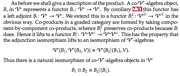
Demonstration of OO in LaTeX

The source for this paragraph begins:

As before we shall give a description of the product.
A \GvCGvobj[\GvCGvobj] represents a functor
 \(\cov{\GvCGvobj} \colon \Gvcat \to \Gvcat\).

Notice how much \GvCGvobj[\GvCGvobj] expands to, and that the outer \GvCGvobj and the inner \GvCGvobj end up as different things.

The point of doing all of this was to achieve consistency throughout the paper (roughly 60 pages) while allowing us (the authors) freedom to change our minds (as we frequently did) as to how things would be rendered. By defining everything in layers, changing the base layer filtered through to the higher layers seamlessly. Note also that in the preamble (well, actually in a style file for ease of maintenance) there are almost 200 calls to the defining \objelt macro (NB the count is done from the version on my computer which may differ from the version on the arXiv).

There are other examples of similar things in that paper. I found this way of defining macros so useful, I used the same or similar scheme in other papers: Comparative Smootheology (arXiv version, published version) and Tall-Wraith Monoids (arXiv version) use exactly the same scheme, then in Yet More Smooth Spaces and Their Smoothly Local Properties (arXiv version) I'd learnt about PGF's OO module and tried using it; my latest version (not available on the web as yet) reimplements it using LaTeX3.

Although it did take time to design this system, and it may well be that the time taken more than compensated for any time saved by using it, it really did help in that it allowed us to truly separate content from style since in the document we could just write the name of the thing and worry about how it would be rendered later. Then, if we didn't like what it looked like, we could change that at a later date and know that the whole document would be consistent (no horrendous search-and-replaces needed).

(As an extreme example, at one point we were undecided as to whether we would write actions on the left or right so built in the ability to swap the entire document from one convention to the other. Fortunately, we realised that that was silly before it got too tangled.)

I think that this is the first time I really programmed a paper. I've since used the programmatic capabilities of (La)TeX many times and in many guises. It's been disallowed by clarification in the comments on the question, but I'm going to sneak in a link to my implementation of Hobby's algorithm and calligraphic library both of which involve more actual programming than, I think, a "normal" LaTeX package generally does. There are others that I could mention, but time and tide have waited long enough ...

0
12

As an academic, I need to maintain multiple versions of my CVs: a full CV with the complete list of publications and grants, CVs for different funding agencies that only require publications and grants from the last 5 or 6 years, an "yearly progress report" for the department with publications and grants in the last year, and so on. Some CV's require the name of the student co-authors to be highlighted, others don't; some require grants to be formatted as a table, others require grants to be highlighted as a itemized list, and so on.

Manually maintaining the multiple versions of these CVs is very time consuming and error-prone task. I automate it as follows:

  1. I have two XML files, publications.xml and grants.xml. These look as follows:
<?xml version="1.0" encoding="UTF-8" ?>
<publication-list>
  <journal-list>
    <publication status="submitted"> 
      <title>
        ...
      </title>
      <authors>
        <name type="student">...</name>
        <name>...</name>
      </authors>
      <journal>
        ...
      </journal>
      <pages>...</pages>
      <month>...</month>
      <year>...</year>
    </publication>

    <publication>
      ...
    </publication>
    ...
  </journal-list>
  <conference-list>
    <publication>
      ...
    </publication>
    ...
  </conference-list>
</publication-list>

and

<?xml version="1.0" encoding="UTF-8" ?>
<grant-list>
  <grant status="applied" type="operational">
    <type>
      ...
    </type>
    <title>
      ...
    </title>
    <authors>
      <name type="PI">...</name>
      <name type="coPI">...</name>
      <name type="coPI">...</name>
    </authors>
    <amount>
      <year year="..." personal="...">...</year>
      <year year="..." personal="...">...</year>
      <year year="..." personal="...">...</year>
    </amount>
  </grant>
  <grant>
    ...
  </grant>
</grant-list>
  1. Relax-NG schemas to validate the XML files.

  2. ConTeXt code that parses the XML files into a Lua table. I use a Lua table as an intermediate because I do not completely understand XML selectors.

  3. ConTeXt Lua Document that takes the data (Lua table) as input and creates appropriatey formatted output

  4. All these files are stored in a Dropbox folder. On my office computer, I run atchange program to monitor the XML files and automatic trigger ConTeXt compilation at any change.

Whenever I need to add anything to my list of publications or grants, I simply edit the XML files on any laptop or desktop. Dropbox syncs all these files, the atchange program compiles everything on my office computer, and I get updated pdf on whichever machine I am using!

It took some time to get this setup right, but now I don't have to worry about keeping multiple CVs in sync. As a by-product, I also generate the list of publications for my homepage using the same setup.

12

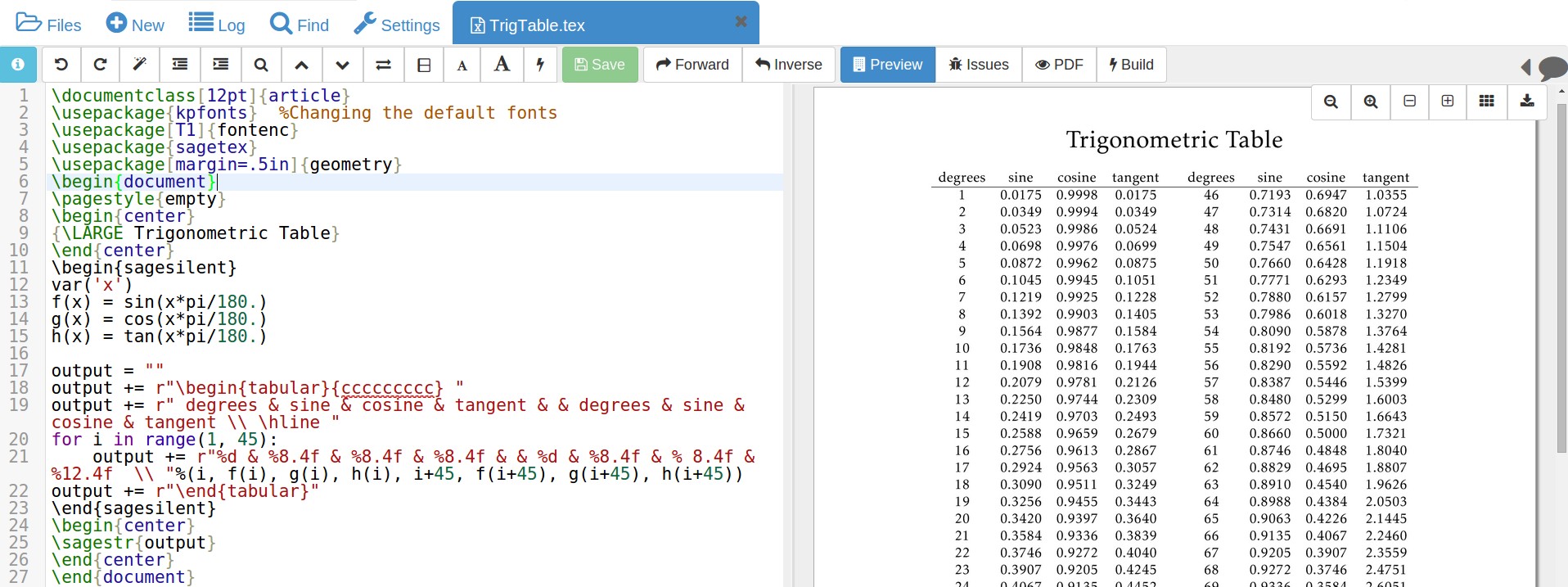
How long would it take you to create this trig table in MS Word? 27 lines of code (counting the blank lines) using LaTeX and sagetex package to make this for my math class.

\documentclass[12pt]{article}
\usepackage{kpfonts}  %Changing the default fonts
\usepackage[T1]{fontenc}
\usepackage{sagetex}
\usepackage[margin=.5in]{geometry}
\begin{document}
\pagestyle{empty}
\begin{center}
{\LARGE Trigonometric Table}
\end{center}
\begin{sagesilent}
var('x')
f(x) = sin(x*pi/180.)
g(x) = cos(x*pi/180.)
h(x) = tan(x*pi/180.)

output = ""
output += r"\begin{tabular}{ccccccccc} "
output += r" degrees & sine & cosine & tangent & & degrees & sine & cosine &  tangent \\ \hline "
for i in range(1, 45):
    output += r"%d & %8.4f & %8.4f & %8.4f & & %d & %8.4f & % 8.4f & %12.4f  \\ "%(i, f(i), g(i), h(i), i+45, f(i+45), g(i+45), h(i+45))
output += r"\end{tabular}"
\end{sagesilent}
\begin{center}
\sagestr{output}
\end{center}
\end{document}

With this output from the code in Sagemath Cloudenter image description here

6
  • 3
    Not that I'm a fan but you would use Excel for this and then copy/paste. Also you can use datatool/pgfplotstable etc. for creating the table locally.
    – percusse
    Commented Dec 29, 2014 at 0:07
  • 1
    Agreed with percusse, and you can use graphical spreadsheet softwares to write this kind of tables in latex too. But since you're bringing sage into the equation, it will not be hard to get out of the reach of excel.
    – T. Verron
    Commented Dec 29, 2014 at 14:02
  • I thought they were comparing LaTeX with other text processors (eg Word). cryingshadows answer above looks like something that could be duplicated with PowerPoint.
    – DJP
    Commented Dec 29, 2014 at 15:24
  • Thanks for pointing package sageTex, I did not know about it. I just tried the example http://www.sagemath.org/doc/tutorial/sagetex.html and it works very well. I think this is the right way to go about it. Now one can write the latex and the computations all in same place. This is much better than using external tools and copy and paste.
    – Nasser
    Commented Dec 30, 2014 at 0:57
  • 1
    @Nasser Yes, computations on the fly and randomization, too. If you do much math it's a must-have package. Documentation is at Ctan. You can search for more sagetex questions at this site or AskSagemath.
    – DJP
    Commented Dec 30, 2014 at 1:27
5

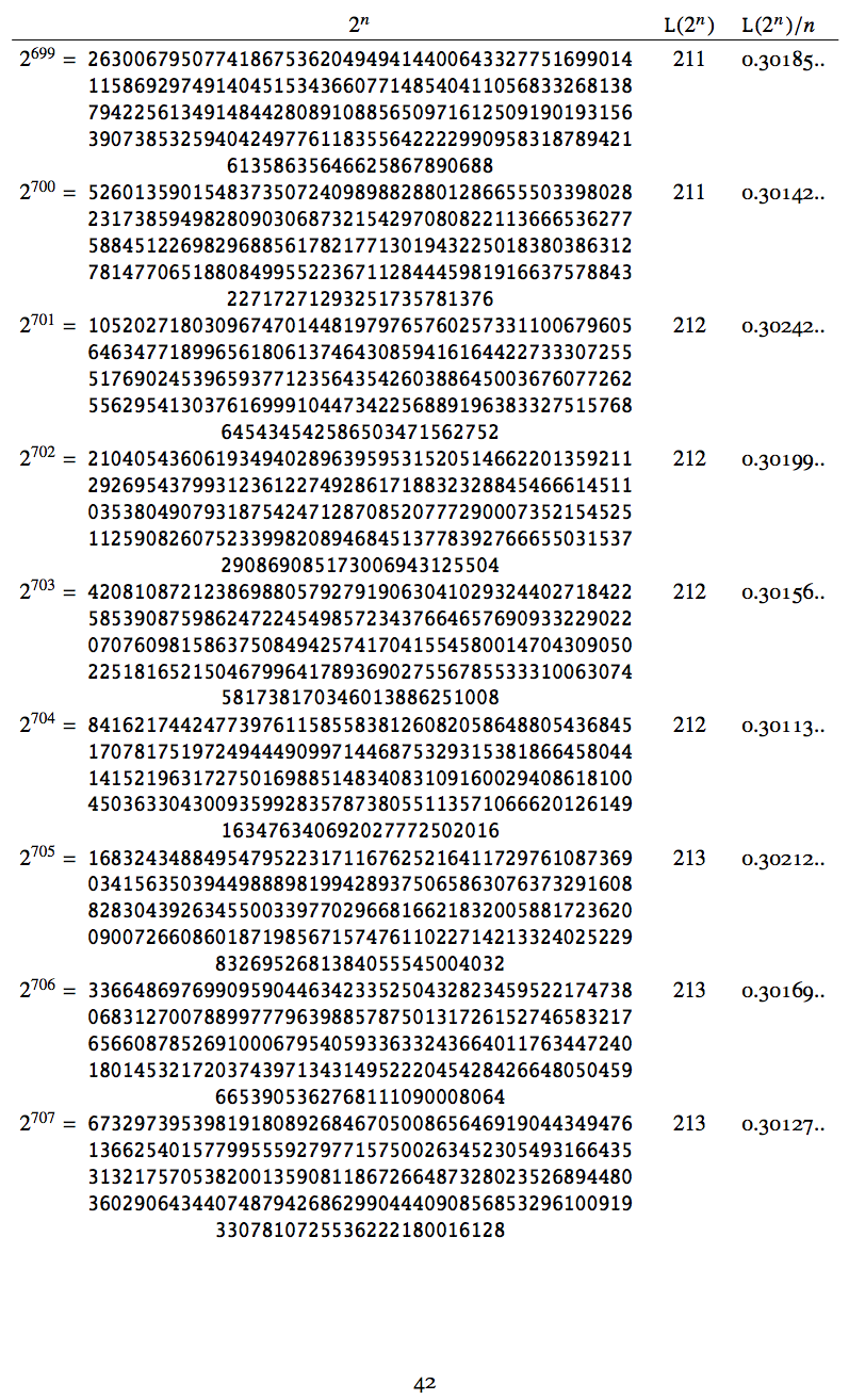
This is a LaTeX file of a few dozen lines which generates an 85 pages document, which consists of a long table where each row contains a power of two 2^n, its length (in base 10), and the ratio length/n with 5 digits after decimal mark. This tends (slowly, hence no need to print more digits...) to a limit the mathematically inclined reader will be able to identify ;-).

Allow a few seconds for compilation (on a contemporary machine). Nothing external to TeX/LaTeX is used (but the e-TeX extensions from 1999 should be available; this is the default in all modern TeX installations).

Here is page 42:

powers of two

The packages used are, mainly:

  1. longtable for the table extending across multiple pages (notice that TeX's original \halign splits with no problem across pages, but not LaTeX's tabular environment)

  2. newtxtext, newtxmath, and newtxtt for fonts. I used old style figures for the length/n ratio, and typewriter style for the powers of 2.

  3. xintfrac and xinttools for the number crunching and table generation.

Other typical packages are used like geometry, hyperref, fontenc, inputenc, and babel. I also needed a few macros to let TeX break big numbers across lines (this is not automatic).

% -*- coding:iso-latin-1; -*-
\documentclass[a4paper]{article}
\usepackage[T1]{fontenc}
\usepackage[latin1]{inputenc}
\usepackage{geometry}

\usepackage[osf]{newtxtext}
\usepackage{newtxmath}
\usepackage{newtxtt}

\usepackage[pdfencoding=pdfdoc]{hyperref}
\hypersetup{%
pdfauthor={jfbu},%
pdftitle={Powers of 2 and their lengths},%
pdfsubject={math stuff, logarithm, powers},%
pdfkeywords={logarithm, powers},%
pdfstartview=FitH,%
pdfpagemode=UseNone}

\usepackage{array}
\usepackage{longtable}
\LTchunksize=100 % don't recall why I did that

\newcounter{index}% counter for use in table generation

\usepackage{xintfrac}% for math and «length»
\usepackage{xinttools}% for \xintloop

\usepackage[french]{babel}
\frenchbsetup{og=«,fg=»}

% macros for splitting across lines big numbers
\def\allowsplits #1{\ifx #1\relax \else #1\hskip 0pt plus 1pt \relax
                    \expandafter\allowsplits\fi}%
\def\printnumber #1{\expandafter\allowsplits \romannumeral-`0#1\relax }%

\let\np\printnumber

\begin{document}

\begin{center}
    \bfseries
    LONGUEURS (en base 10) DES $2^n$ jusqu'à $n=1024$\par
\end{center}

% a long table with four columns

\begin{longtable}{@{}r@{}>{\centering\ttfamily}p{.6\linewidth}cl}
%% header
    &$2^n$&$\texttt{L}(2^n)$&$\texttt{L}(2^n)/n$\\
    \hline
    \noalign{\vskip\jot}\endhead
%% first row after head:
    \setcounter{index}{0}% automatically global, hence ok from cell to cell
    \gdef\PowerOfTwo {1}%
     $2^0 ={}$& % first cell
     1&         % second cell, containing power of two
     $1$&       % third cell, containing length of power of two in base 10
     \np{1.00000}..\\ % 2^0=1
%% next 1024 rows:
    \xintloop 
          \stepcounter{index}%
          \global\oodef\PowerOfTwo {\xintDouble\PowerOfTwo }%
          \gdef\LenPowerTwo        {\xintLen\PowerOfTwo }%
    % %
          $2^{\arabic{index}}={}$ &
          \np{\PowerOfTwo}   &
          $\LenPowerTwo$     &
          \np{\xintTrunc {5}{\LenPowerTwo/\value{index}}}..\\
    \unless\ifnum\value{index}=1024
    \repeat
    \hline
\end{longtable}

\end{document}
2

AUCTeX's preview-latex contains circ.tex in its distribution which illustrates various digital differential algorithms in diagrams generated with straightforward TeX programming (as opposed to various external systems like PostScript or Lua or Sage used in some other answers).

You must log in to answer this question.

Not the answer you're looking for? Browse other questions tagged .